The Maths Behind Image Compression

You've probably seen an image that looks like this before

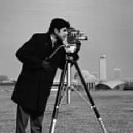
If you look closely, you can see the image is broken up into multiple blocks, which seem to have patterns inside them

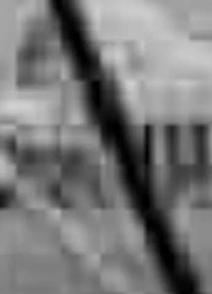
This is the result of JPEG image compression (Computerphile, 2015). JPEG is a lossy format, meaning it can reduce file size by discarding some visual information that is less noticeable to the human eye. But why does it make the image look like this?

And more importantly, how does it relate to trigonometry?

Why we need trigonometry to compress an image

Fundamentally, lossy JPEG image compression is quite a simple concept. It reduces image detail that is less important to how we see the image. But to do that, the image first needs to be converted into a format where that detail is easier reduce.

That's why the Discrete Cosine Transform (DCT) is used to compress images. The DCT is a way of expressing data as a sum of cosine functions. It's similar to the Fourier Transform , but only uses cosine functions (Wikipedia Contributors, 2020).

While not compressing the image itself, the DCT makes it a lot easier to compress images, by rearranging image data, so that most of the visually important information is represented in a small number of low-frequency coefficients. JPEG can then store the image more efficiently by removing/reducing the higher-frequency coefficients.

A way to think about this is that an image isn't only pixels, but also patterns. Some patterns change slowly, like smooth gradients, while others change quickly, like sharp edges, fine texture, or noise.

Trig functions are useful because they let us describe these patterns by frequency. A low frequency cosine wave changes slowly, while a high frequency cosine wave changes quickly. By combining multiple cosine waves, we can represent complex data, including brightness values in an image.

In this simple model, k controls the frequency. When k is small, the graph changes slowly. When k is larger, the graph oscillates more often over the same interval.

The graph below shows this idea in one dimension. As the frequency changes, the wave oscillates more or less rapidly. JPEG applies the same idea to small two-dimensional blocks of image data.

This graph supports the compression model because it shows how frequency changes the shape of a cosine wave. In an image, low-frequency cosine patterns represent smooth changes in brightness, while high-frequency cosine patterns represent sudden changes such as edges, fine texture, and noise.

So we've discussed the idea. Now time to apply it.

Compressing an Image

Let's take an example. I'll be using a simple black and white image for now:

Preparation

To compress this image, it is first split into 8x8 blocks (Wikipedia Contributors, 2019b). This makes it easier to work with, and can allow the image to be compressed more efficiently. A compressor will then loop over each block compressing it separately.

Let's take this part of the image and work with that

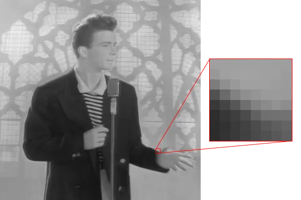
Firstly, we can take the brightness of each pixel from 0 - 255 and represent it as a grid:

Then we need to shift the values to be around 0. JPEG does this by subtracting 128 from each pixel:

Now we need to express this block as a weighted sum of cosine patterns. This is where trigonometry comes in.

This is a plot of 64 cosine patterns, one for each value in an 8x8 block:

These patterns are usually called the DCT basis functions. Each square above is a graphical model of one two-dimensional cosine pattern. The grid shows why the DCT is connected to trigonometry. The image block is rebuilt by adding these cosine patterns together with different weights. The top-left pattern is constant, while patterns further right and further down oscillate more quickly.

• The top-left square is lowest frequency
• Moving right increases horizontal frequency
• Moving down increases vertical frequency
• The bottom-right square is highest frequency in both directions

But how is this useful? With these 64 basis functions, we can represent any 8x8 block of pixel values. The DCT tells us how much of each basis function is needed.

After the DCT is applied, we get another 8x8 grid. But these numbers aren't pixel brightness, they are coefficients, telling us how strongly each function appears in the block.

The top left coefficient, called the DC coefficient is responsible for storing the average brightness of the 8x8 block. The remaining coefficients are called AC coefficients and describe changes in brightness across the block.

You can see in this example, the second coefficient from the top (the one at 287) is pretty high, indicating that the function appears strongly in the block.

In most images, nearby pixels are similar. This means a lot of the important information in the image is stored in the lower frequency coefficients (the ones up the top left of the DCT grid), while the higher frequency coefficients are mostly unimportant details.

These details are removed using a quantisation table, which is an 8x8 table specifying the values to divide each coefficient by before storing it. The values are then rounded to the nearest integer. This is the main lossy step in JPEG's DCT-based process, because rounding changes the coefficients and loses some exact detail.

Large divisors make coefficients more likely to round to zero, which is where file size drops and detail is reduced. This is because zeros are a lot easier to compress than non-zero values.

Then the process is repeated on each 8x8 block of the image.

Why I Chose This Application

I chose image compression because it is a practical use of trigonometry that appears constantly in everyday technology. I'm also interested in tech, and wanted to do something tech related. I found the method JPEG uses to compress images to be fascinating, and wanted to explore it further.

Conclusion

I think image compression is an interesting use of trigonometry, and I had fun researching and trying to understand how two seemingly unrelated things are actually related.

I hope you learned something :)

References

Computerphile. (2015). JPEG DCT, Discrete Cosine Transform (JPEG Pt2)- Computerphile [YouTube Video]. In YouTube. https://www.youtube.com/watch?v=Q2aEzeMDHMA
Discrete Cosine Transform - MATLAB & Simulink - MathWorks Australia. (n.d.). Au.mathworks.com. https://au.mathworks.com/help/images/discrete-cosine-transform.html
Swanson, J. (n.d.). An Interactive Introduction to Fourier Transforms. Www.jezzamon.com. https://www.jezzamon.com/fourier/
Wikipedia Contributors. (2019a, June 26). Data compression. Wikipedia; Wikimedia Foundation. https://en.wikipedia.org/wiki/Data_compression
Wikipedia Contributors. (2019b, October 8). JPEG. Wikipedia; Wikimedia Foundation. https://en.wikipedia.org/wiki/JPEG
Wikipedia Contributors. (2020, August 10). Discrete cosine transform. Wikipedia. https://en.wikipedia.org/wiki/Discrete_cosine_transform